44 data labels excel 2013

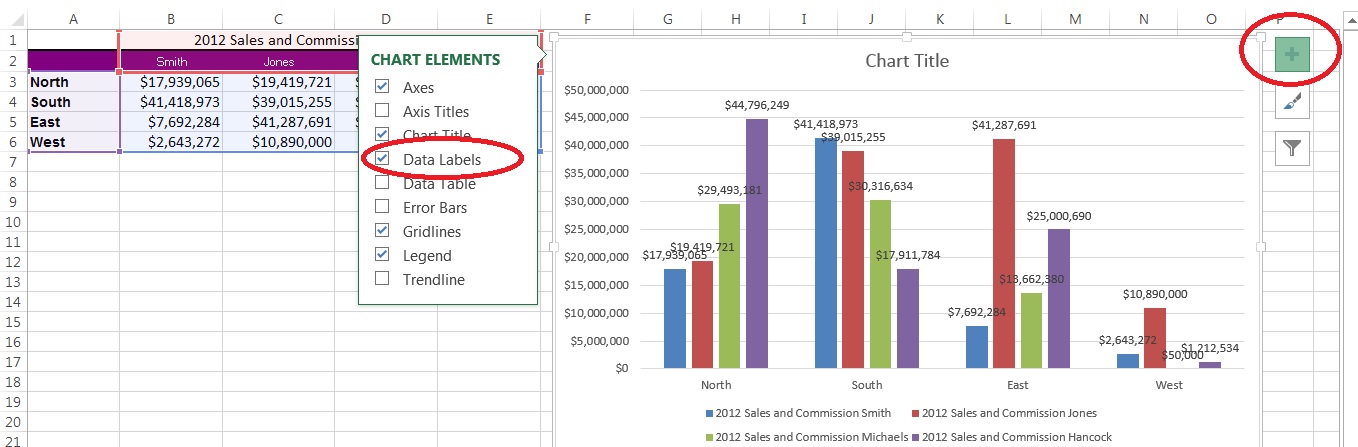
Reddit - Dive into anything Value From Cells data label in Excel 2013 is not backwards-compatible unsolved I was excited to see that Excel 2013 lets me use a range cell values for data labels in XY charts. (They are located in Label Options). Previously, I had resorted to the XY label add-in that every Excel scatterplotter eventually discovers. How to Add Data Labels in Excel - Excelchat | Excelchat How to Add Data Labels In Excel 2013 And Later Versions In Excel 2013 and the later versions we need to do the followings; Click anywhere in the chart area to display the Chart Elements button Figure 5. Chart Elements Button Click the Chart Elements button > Select the Data Labels, then click the Arrow to choose the data labels position. Figure 6.

Introduction to the Data Model and Relationships in Excel 2013 ... In Excel, go to the DATA tab and select "From Other Sources", "From Windows Azure Marketplace". Fill out the information with what you have saved from the website: Select that table. Hit "Finish" and then select "Only Create Connection": Note: Some of you might be wondering why I chose "Only Create Connection".

Data labels excel 2013

Adding Data Labels to Your Chart (Microsoft Excel) To add data labels in Excel 2013 or Excel 2016, follow these steps: Activate the chart by clicking on it, if necessary. Make sure the Design tab of the ribbon is displayed. (This will appear when the chart is selected.) Click the Add Chart Element drop-down list. Select the Data Labels tool. How to add or move data labels in Excel chart? - ExtendOffice To add or move data labels in a chart, you can do as below steps: In Excel 2013 or 2016. 1. Click the chart to show the Chart Elements button .. 2. Then click the Chart Elements, and check Data Labels, then you can click the arrow to choose an option about the data labels in the sub menu.See screenshot: How to Create and Label a Pie Chart in Excel 2013 Open Microsoft Excel 2013 and click on the "Blank workbook" option. Add Tip Ask Question Comment Download Step 2: Input the Data Create your spreadsheet by inputting the numbers and labels which are going to be used in the pie chart. In this example, I used the labels "Desserts", "Appertizers", "Entrees", "Beer", and "Wine". Add Tip Ask Question

Data labels excel 2013. How to Insert Axis Labels In An Excel Chart | Excelchat Figure 8 - How to edit axis labels in Excel. Add Axis Label in Excel 2016/2013. In Excel 2016 and 2013, we have an easier way to add axis labels to our chart. We will click on the Chart to see the plus sign symbol at the corner of the chart; Figure 9 - Add label to the axis We will click on the plus sign to view its hidden menu . Here, we ... How to Add Data Labels to your Excel Chart in Excel 2013 Data labels show the values next to the corresponding chart element, for instance a percentage next to a piece from a pie chart, or a total value next to a column in a column chart. You can choose... Apply Custom Data Labels to Charted Points - Peltier Tech For data labels, the best tool by far is the XY chart label add in. I have Excel 2013 and have found that the Excel linked labels are not as reliable when the cells change as Rob Bovey's add in. Excel is complicated enough. We don't need to add complexity. Cheers, Excel 2013 Graphs automatically aligning data labels to end of bar Posts: 14. Excel 2013 Graphs automatically aligning data labels to end of bar. Hi. In Excel 2013 I am wanting to align the data labels in a graph automatically to be at the end of the bar (in a bar graph obviously). I know how to move them manually, but I remember there used to be a way to make it move them all automatically.

Creating a chart with dynamic labels - Microsoft Excel 2013 Excel 2013 365 2016. This tip shows how to create dynamically updated chart labels that depend on value or other cells. ... For all labels: on the Format Data Labels task pane, in the Label Options, in the Label Contains group, check Value From Cells and then choose cells: Values From Cell: Missing Data Labels Option in Excel 2013? 8. May 27, 2015. #1. Ive inherited a Powerpoin with an embedded Excel chart and data sheet. The graph in Powerpoint shows several instances of a value [CellRange]. Im trying to figure out where its "trying" to pull its data from and I think because the data is not in a contiguous range its having trouble. A couple articles refer to formatting ... Values From Cell: Missing Data Labels Option in Excel 2013? When a chart created in 2013 using the "Values from Cell" data label option is opened with any earlier version of Excel, the data labels will show as " [CELLRANGE]". If you want to ensure that data labels survive different generations of Excel, you need to revert to the old technique: Insert data labels Edit each individual data label How to Print Labels from Excel - Lifewire Choose Start Mail Merge > Labels . Choose the brand in the Label Vendors box and then choose the product number, which is listed on the label package. You can also select New Label if you want to enter custom label dimensions. Click OK when you are ready to proceed. Connect the Worksheet to the Labels

Custom Data Labels with Colors and Symbols in Excel Charts - [How To] To apply custom format on data labels inside charts via custom number formatting, the data labels must be based on values. You have several options like series name, value from cells, category name. But it has to be values otherwise colors won't appear. Symbols issue is quite beyond me. How to add data labels from different column in an Excel chart? Right click the data series in the chart, and select Add Data Labels > Add Data Labels from the context menu to add data labels. 2. Click any data label to select all data labels, and then click the specified data label to select it only in the chart. 3. Change the format of data labels in a chart To get there, after adding your data labels, select the data label to format, and then click Chart Elements > Data Labels > More Options. To go to the appropriate area, click one of the four icons ( Fill & Line, Effects, Size & Properties ( Layout & Properties in Outlook or Word), or Label Options) shown here. Excel Tips n Tricks -Tip 8 (Applying Chart Data Labels From a Range in ... Click on the plus symbol, the first icon, and check "Data Labels". Now you will see them added to your chart. You can also click on the right arrow on "Data Labels" and select where you want the data labels to be aligned, in other words center, right, top, bottom and so on. Picture 4 4. I modified the chart and axis titles to look good.

Label Template Excel | printable label templates

Excel 2013 Chart Labels don't appear properly - Microsoft Community You've stumbled on a big problem - Excel 2013 lets you edit data labels directly, but this feature (rich text data labels) is not backwards-compatible and there's no way to turn it off. It's great to be able to modify the text of labels, or direct them to get contents from a worksheet cell.

Changing Axis Labels in PowerPoint 2011 for Mac

Add or remove data labels in a chart - support.microsoft.com Right-click the data series or data label to display more data for, and then click Format Data Labels. Click Label Options and under Label Contains, select the Values From Cells checkbox. When the Data Label Range dialog box appears, go back to the spreadsheet and select the range for which you want the cell values to display as data labels.

Format Data Labels in Excel- Instructions | Microsoft excel, Microsoft, Bar chart

Adding rich data labels to charts in Excel 2013 - Microsoft 365 Blog You can do this by adjusting the zoom control on the bottom right corner of Excel's chrome. Then, select the value in the data label and hit the right-arrow key on your keyboard. The story behind the data in our example is that the temperature increased significantly on Wednesday and that appeared to help drive up business at the lemonade stand.

Microsoft Tips with Temo!: How to Add Data Labels to an Excel 2010 Chart

formatting - How to format Microsoft Excel data labels without trailing ... To get this to work, I formatted the cell's of the data column 4 4 4 4 3.5 13.5, by either selecting the column and then right click and format cells or by right clicking on the chart and selecting format data labels.I formatted this with the regular expression $#K so that the data then shows as $4K $4K $4K $4K $4K $14K. The consequence is that the number is rounded to not include the decimal.

Advanced Graphs Using Excel : Shading under a distribution curve (eg. normal curve) in excel

How to Use Cell Values for Excel Chart Labels Select the chart, choose the "Chart Elements" option, click the "Data Labels" arrow, and then "More Options.". Uncheck the "Value" box and check the "Value From Cells" box. Select cells C2:C6 to use for the data label range and then click the "OK" button. The values from these cells are now used for the chart data labels.

30 What Is A Data Label In Excel - Labels Database 2020

How to Add Total Data Labels to the Excel Stacked Bar Chart Step 4: Right click your new line chart and select "Add Data Labels" Step 5: Right click your new data labels and format them so that their label position is "Above"; also make the labels bold and increase the font size. Step 6: Right click the line, select "Format Data Series"; in the Line Color menu, select "No line"

How to Make Charts and Graphs in Excel | Smartsheet

How to Customize Chart Elements in Excel 2013 - dummies To add data labels to your selected chart and position them, click the Chart Elements button next to the chart and then select the Data Labels check box before you select one of the following options on its continuation menu: Center to position the data labels in the middle of each data point

30 How To Add Label To Excel Chart - Labels Database 2020

Quick Tip: Excel 2013 offers flexible data labels | TechRepublic right-click and choose Insert Data Label Field. In the next dialog, select [Cell] Choose Cell. When Excel displays the source dialog, click the cell that contains the MIN () function, and click OK....

Excel 2013 Tutorial Formatting Data Labels Microsoft Training Lesson 28.6 - YouTube

How to insert data labels to a Pie chart in Excel 2013 - YouTube This video will show you the simple steps to insert Data Labels in a pie chart in Microsoft® Excel 2013. Content in this video is provided on an "as is" basi...

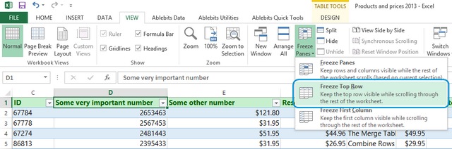
How to keep header rows in Excel visible

Label Options for Chart Data Labels in PowerPoint 2013 for Windows The selection is also reflected within the Data Label Range dialog box. Click the OK button when you are done to see the result within the chart's data labels, as shown in Figure 3, below. Figure 3: Alphabets taken from Excel cells added as part of the data label ; Series Name ; Displays name of the series in data labels. Category Name

How to sort in Excel Tables

How to Create and Label a Pie Chart in Excel 2013 Open Microsoft Excel 2013 and click on the "Blank workbook" option. Add Tip Ask Question Comment Download Step 2: Input the Data Create your spreadsheet by inputting the numbers and labels which are going to be used in the pie chart. In this example, I used the labels "Desserts", "Appertizers", "Entrees", "Beer", and "Wine". Add Tip Ask Question

Format Number Options for Chart Data Labels in Excel 2011 for Mac

How to add or move data labels in Excel chart? - ExtendOffice To add or move data labels in a chart, you can do as below steps: In Excel 2013 or 2016. 1. Click the chart to show the Chart Elements button .. 2. Then click the Chart Elements, and check Data Labels, then you can click the arrow to choose an option about the data labels in the sub menu.See screenshot: