42 data labels on excel chart
How To Use Dynamic Data Labels To Create Interactive Excel Charts To create a column chart with dynamic data labels, you need to follow these given steps. Select the data & Create a Combo Chart. Now select the column chart for revenue data and a line chart with marker for data labels Add Data Labels to the Line Chart With Marker. After then remove the Line Color and Marker Color. Custom Chart Data Labels In Excel With Formulas Follow the steps below to create the custom data labels. Select the chart label you want to change. In the formula-bar hit = (equals), select the cell reference containing your chart label's data. In this case, the first label is in cell E2. Finally, repeat for all your chart laebls.
How to Add Data Labels in Excel - Excelchat | Excelchat After inserting a chart in Excel 2010 and earlier versions we need to do the followings to add data labels to the chart; Click inside the chart area to display the Chart Tools. Figure 2. Chart Tools Click on Layout tab of the Chart Tools. In Labels group, click on Data Labels and select the position to add labels to the chart. Figure 3.

Data labels on excel chart
How to add data labels from different column in an Excel chart? Right click the data series in the chart, and select Add Data Labels > Add Data Labels from the context menu to add data labels. 2. Click any data label to select all data labels, and then click the specified data label to select it only in the chart. 3. Add data labels and callouts to charts in Excel 365 | EasyTweaks.com Excel also gives you the option of formatting the data labels to suit your desired look if you don't like the default. To make changes to the data labels, right-click within the chart and select the "Format Labels" option. Some of the formatting options you will have include; changing the label position, changing its alignment angle, and many more. Add / Move Data Labels in Charts - Excel & Google Sheets Adding Data Labels Click on the graph Select + Sign in the top right of the graph Check Data Labels Change Position of Data Labels Click on the arrow next to Data Labels to change the position of where the labels are in relation to the bar chart Final Graph with Data Labels
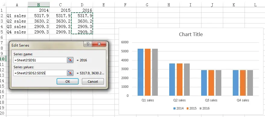
Data labels on excel chart. Chart.ApplyDataLabels method (Excel) | Microsoft Docs Syntax expression. ApplyDataLabels ( Type, LegendKey, AutoText, HasLeaderLines, ShowSeriesName, ShowCategoryName, ShowValue, ShowPercentage, ShowBubbleSize, Separator) expression A variable that represents a Chart object. Parameters Example This example applies category labels to series one on Chart1. VB Copy Charts ("Chart1").SeriesCollection (1). How to Add Data Labels to an Excel 2010 Chart - dummies Use the following steps to add data labels to series in a chart: Click anywhere on the chart that you want to modify. On the Chart Tools Layout tab, click the Data Labels button in the Labels group. None: The default choice; it means you don't want to display data labels. Center to position the data labels in the middle of each data point. How to add total labels to stacked column chart in Excel? 1. Create the stacked column chart. Select the source data, and click Insert > Insert Column or Bar Chart > Stacked Column. 2. Select the stacked column chart, and click Kutools > Charts > Chart Tools > Add Sum Labels to Chart. Then all total labels are added to every data point in the stacked column chart immediately. Adding Data Labels to Your Chart (Microsoft Excel) To add data labels, follow these steps: Activate the chart by clicking on it, if necessary. Choose Chart Options from the Chart menu. Excel displays the Chart Options dialog box. Make sure the Data Labels tab is selected. (See Figure 1.) The left side of the dialog box shows the different types of data labels you can choose. (The available ...
Move data labels - support.microsoft.com Click any data label once to select all of them, or double-click a specific data label you want to move. Right-click the selection > Chart Elements > Data Labels arrow, and select the placement option you want. Different options are available for different chart types. How to Use Cell Values for Excel Chart Labels Select the chart, choose the "Chart Elements" option, click the "Data Labels" arrow, and then "More Options.". Uncheck the "Value" box and check the "Value From Cells" box. Select cells C2:C6 to use for the data label range and then click the "OK" button. The values from these cells are now used for the chart data labels. Add data labels to your Excel bubble charts | TechRepublic Follow these steps to add the employee names as data labels to the chart: Right-click the data series and select Add Data Labels. Right-click one of the labels and select Format Data Labels. Select... Edit titles or data labels in a chart - support.microsoft.com On a chart, click one time or two times on the data label that you want to link to a corresponding worksheet cell. The first click selects the data labels for the whole data series, and the second click selects the individual data label. Right-click the data label, and then click Format Data Label or Format Data Labels.
Add or remove data labels in a chart - support.microsoft.com Click the data series or chart. To label one data point, after clicking the series, click that data point. In the upper right corner, next to the chart, click Add Chart Element > Data Labels. To change the location, click the arrow, and choose an option. If you want to show your data label inside a text bubble shape, click Data Callout. Excel tutorial: How to use data labels When you check the box, you'll see data labels appear in the chart. If you have more than one data series, you can select a series first, then turn on data labels for that series only. You can even select a single bar, and show just one data label. In a bar or column chart, data labels will first appear outside the bar end. How to add or move data labels in Excel chart? - ExtendOffice In Excel 2013 or 2016. 1. Click the chart to show the Chart Elements button . 2. Then click the Chart Elements, and check Data Labels, then you can click the arrow to choose an option about the data labels in the sub menu. See screenshot: In Excel 2010 or 2007. 1. click on the chart to show the Layout tab in the Chart Tools group. See ... How to I rotate data labels on a column chart so that they are ... To change the text direction, first of all, please double click on the data label and make sure the data are selected (with a box surrounded like following image). Then on your right panel, the Format Data Labels panel should be opened. Go to Text Options > Text Box > Text direction > Rotate

Multiple Series in One Excel Chart - Peltier Tech Blog
Adding Data Labels to Your Chart (Microsoft Excel) To add data labels in Excel 2013 or Excel 2016, follow these steps: Activate the chart by clicking on it, if necessary. Make sure the Design tab of the ribbon is displayed. (This will appear when the chart is selected.) Click the Add Chart Element drop-down list. Select the Data Labels tool.

Nested donut chart (also known as Multi-level doughnut chart, Multi-series doughnut chart ...
Excel Charts - Aesthetic Data Labels - Tutorials Point Data labels stay in place, even when you switch to a different type of chart. You can also connect the data labels to their data points with leader lines on all charts. Here, we will use a Bubble chart to see the formatting of data labels. Data Label Positions. To place the data labels in the chart, follow the steps given below.
Charts and Graphs in Excel
Adding rich data labels to charts in Excel 2013 - Microsoft 365 Blog Putting a data label into a shape can add another type of visual emphasis. To add a data label in a shape, select the data point of interest, then right-click it to pull up the context menu. Click Add Data Label, then click Add Data Callout . The result is that your data label will appear in a graphical callout.
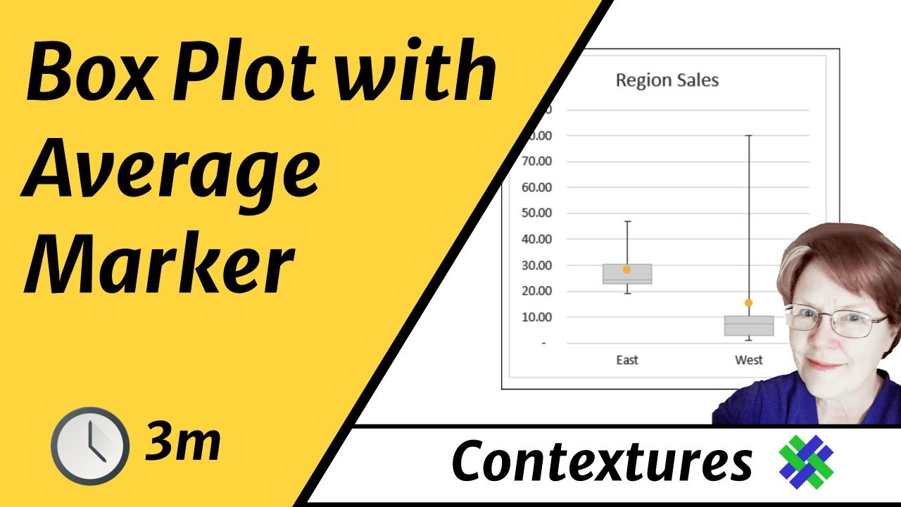
Add Average Marker to Excel Box Plot - Box and Whisker Chart - YouTube
Add a DATA LABEL to ONE POINT on a chart in Excel Click on the chart line to add the data point to. All the data points will be highlighted. Click again on the single point that you want to add a data label to. Right-click and select ' Add data label ' This is the key step! Right-click again on the data point itself (not the label) and select ' Format data label '.
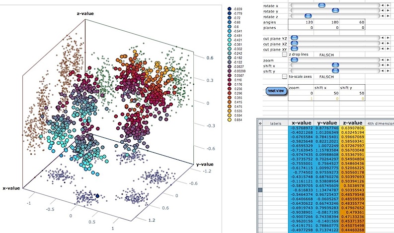
3d scatter plot for MS Excel
Use a screen reader to add a title, data labels, and a legend to a ... Select the chart that you want to work with. To open the Add Chart Element menu, press Alt+J, C, A. To add data callout labels to the chart, press D and then U. Tip: To remove data labels, select the chart, and then press Alt+J, C, A, D, and then N. Add a legend to a chart Legends help you to quickly understand data relationships in a chart.

Bar charts with long category labels; Issue #428 November 27 2018 | Think Outside The Slide
Excel charts: how to move data labels to legend - Microsoft Tech Community You can't do that, but you can show a data table below the chart instead of data labels: Click anywhere on the chart. On the Design tab of the ribbon (under Chart Tools), in the Chart Layouts group, click Add Chart Element > Data Table > With Legend Keys (or No Legend Keys if you prefer)
Excel clustered column chart - Access-Excel.Tips
Excel Chart Data Labels - Microsoft Community Please verify that the range of data labels has been selected correctly. Right-click a data point on your chart, from the context menu choose Format Data Labels ..., choose Label Options > Label Contains Value from Cells > Select Range. In the Data Label Range dialog box, verify that the range includes all 26 cells.
Excel Gantt Chart - Free Excel Templates
How to create Custom Data Labels in Excel Charts Add data labels Create a simple line chart while selecting the first two columns only. Now Add Regular Data Labels. Two ways to do it. Click on the Plus sign next to the chart and choose the Data Labels option. We do NOT want the data to be shown. To customize it, click on the arrow next to Data Labels and choose More Options …
Post a Comment for "42 data labels on excel chart"